
|
Active Appearance Models (AAM) |
Active Appearance Models (AAM) is a statistical based template matching method, where the variability of shape and texture is captured from a representative training set. Principal Components Analysis (PCA) on shape and texture data allow building a parametrized face model that fully describe with photorealistic quality the trained faces as well as unseen.
Shape Model
The shape is defined as the quality of a configuration of points which is invariant under Euclidian Similarity transformations. This landmark points are selected to match borders, vertexes, profile points, corners or other features that describe the shape. The representation used for a single ![]() -point shape is a
-point shape is a ![]() vector given by
vector given by ![]() . With
. With ![]() shape annotations, follows a statistical analysis where the shapes are previously aligned to a common mean shape using a Generalised Procrustes Analysis (GPA) removing location, scale and rotation effects. Optionally, we could project the shape distribution into the tangent plane, but omitting this projection leads to very small changes. Applying a Principal Components Analysis (PCA), we can model the statistical variation with
shape annotations, follows a statistical analysis where the shapes are previously aligned to a common mean shape using a Generalised Procrustes Analysis (GPA) removing location, scale and rotation effects. Optionally, we could project the shape distribution into the tangent plane, but omitting this projection leads to very small changes. Applying a Principal Components Analysis (PCA), we can model the statistical variation with
Texture Model
For ![]() pixels sampled, the texture is represented by the vector
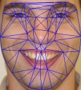
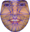
pixels sampled, the texture is represented by the vector ![]() . Building a statistical texture model, requires warping each training image so that the control points match those of the mean shape. In order to prevent holes, the texture mapping is performed using the reverse map with bilinear interpolation correction. The texture mapping is performed, using a piece-wise affine warp, i.e. partitioning the convex hull of the mean shape by a set of triangles using the Delaunay triangulation. Each pixel inside a triangle is mapped into the correspondent triangle in the mean shape using barycentric coordinates, see figure.
. Building a statistical texture model, requires warping each training image so that the control points match those of the mean shape. In order to prevent holes, the texture mapping is performed using the reverse map with bilinear interpolation correction. The texture mapping is performed, using a piece-wise affine warp, i.e. partitioning the convex hull of the mean shape by a set of triangles using the Delaunay triangulation. Each pixel inside a triangle is mapped into the correspondent triangle in the mean shape using barycentric coordinates, see figure.
|
Combined Model
The shape and texture from any training example is described by the parameters ![]() and
and ![]() . To remove correlations between shape and texture model parameters a third PCA is performed to the following data,
. To remove correlations between shape and texture model parameters a third PCA is performed to the following data,
 , where
 ![]() is a diagonal matrix of weights that measures the unit difference between shape and texture parameters. A simple estimate for
is a diagonal matrix of weights that measures the unit difference between shape and texture parameters. A simple estimate for ![]() is to weight uniformly with ratio,
is to weight uniformly with ratio, ![]() , of the total variance in texture and shape, i.e.
, of the total variance in texture and shape, i.e. ![]() , where
, where ![]() and
and ![]() are shape and texture eigenvalues, respectively. Then
are shape and texture eigenvalues, respectively. Then ![]() . As a result, using again a PCA,
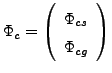
. As a result, using again a PCA, ![]() holds the
holds the ![]() highest eigenvectors, and we obtain the combined model,
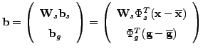
highest eigenvectors, and we obtain the combined model, ![]() . Due the linear nature for the model, it is possible to express shape,
. Due the linear nature for the model, it is possible to express shape, ![]() , and texture,
, and texture, ![]() , using the combined model by
, using the combined model by
 and
and Model Training
An AAM search seek to minimize the texture difference between a model instance and the beneath part of the target image that it covers. It can be treated as an optimization problem where ![]() updating the appearance parameters
updating the appearance parameters ![]() and pose. This nonlinear problem can be solved by learning offline how the model behaves due parameters change and the correspondent relations between the texture residual. Additionally, similarity parameters are considered to represent the 2D pose,
and pose. This nonlinear problem can be solved by learning offline how the model behaves due parameters change and the correspondent relations between the texture residual. Additionally, similarity parameters are considered to represent the 2D pose, ![]() . To maintain linearity and for zero parameters value represent no change in pose, these parameters are redefined to
. To maintain linearity and for zero parameters value represent no change in pose, these parameters are redefined to ![]() ,
, ![]() which represents a combined scale,
which represents a combined scale, ![]() , and rotation,
, and rotation, ![]() , while the remaining parameters
, while the remaining parameters ![]() and
and ![]() are translations. The complete model parameters include also pose,
are translations. The complete model parameters include also pose, ![]() . The initial AAM formulation uses the Multivariate Linear Regression (MLR) approach over the set of training texture residuals,
. The initial AAM formulation uses the Multivariate Linear Regression (MLR) approach over the set of training texture residuals, ![]() , and the correspondent model perturbations,
, and the correspondent model perturbations, ![]() . Assuming that the correlation of texture difference and model parameters update is locally linear, the goal is to get the optimal prediction matrix, in the least square sense, satisfying the linear relation,
. Assuming that the correlation of texture difference and model parameters update is locally linear, the goal is to get the optimal prediction matrix, in the least square sense, satisfying the linear relation, ![]() . Solving it involves perform a set experiences, building huge residuals matrices and perform MLR on these. It was suggested that appearance parameters,
. Solving it involves perform a set experiences, building huge residuals matrices and perform MLR on these. It was suggested that appearance parameters, ![]() , should be perturbed in about
, should be perturbed in about ![]() and
and ![]() . Scale around 90%, 110%, rotation
. Scale around 90%, 110%, rotation ![]() ,
, ![]() and translations
and translations ![]() ,
, ![]() , all with respect to the reference mean frame.
The MLR was later replaced by a simpler approach, computing the gradient matrix,
, all with respect to the reference mean frame.
The MLR was later replaced by a simpler approach, computing the gradient matrix, ![]() , requiring much less memory and computational effort. The texture residual vector is defined as
, requiring much less memory and computational effort. The texture residual vector is defined as ![]() , where the goal is to find the optimal update at model parameters to minimize
, where the goal is to find the optimal update at model parameters to minimize ![]() .
Expanding the texture residuals,
.
Expanding the texture residuals, ![]() , in Taylor series around
, in Taylor series around ![]() and holding the first order terms,
and holding the first order terms, ![]() where
where  is the Jacobian matrix. Differentiating w.r.t.
 ![]() and equalling to zero leads to
and equalling to zero leads to ![]() .
Normally steepest descent approaches require the Jacobian evaluation for each iteration. Since the AAM framework works on a normalize reference frame, the Jacobian matrix can be considered fixed over the training set and can be estimated once on the training phase.
.
Normally steepest descent approaches require the Jacobian evaluation for each iteration. Since the AAM framework works on a normalize reference frame, the Jacobian matrix can be considered fixed over the training set and can be estimated once on the training phase.
Model Fitting
The model parameters are updated over texture residuals by,


|